Isolation Forest(アイソレーションフォレスト)は、機械学習の異常検知手法の一つで、特に大量のデータから異常なデータポイントを効率的に検出できることで注目されています。
このアルゴリズムは、データの「孤立度」を基に異常を検知するユニークなアプローチを取っています。
製造業においても、Isolation Forestは品質管理や設備保全の異常を早期に発見する手段として活用されており、従来の手法では見逃されやすい異常を見つけることが可能です。
この記事では、Isolation Forestの概要から製造業での応用、具体的な実装方法まで、詳しく解説します。
Isolation Forestとは?
Isolation Forestは、異常検知のためのアルゴリズムであり、データの孤立度を利用して異常を特定します。
Isolation Forestは決定木を多数生成し、各データポイントがどれだけ簡単に他のデータから分離できるか(孤立できるか)を評価します。
一般的に、異常なデータポイントは少数派であり、通常のデータと比べて早く孤立されるため、短い経路で検出されます。
メリット
- 高効率・高速処理:大規模なデータセットでも迅速に処理できる。
- 前処理が少ない:従来の異常検知手法と比べ、データの前処理がほとんど必要ない。
- ノンパラメトリック:分布に依存せず、汎用性が高い。
- スケーラビリティ:大量のデータにも適応しやすく、異常を効果的に見つけることができる。
従来の距離ベースの手法(k-NNなど)とは異なり、決定木による分割を行うため、各特徴量のスケール(値の大きさ)を揃える標準化(StandardScalerなど)をせずとも正しく動作します。 異なる単位のセンサー値が混在する製造現場のデータには非常に大きなメリットです。
デメリット
- 解釈性の低さ:異常の原因が特定しにくいことがある。
- 高次元データに弱い:次元が多いデータに対しては精度が低下する可能性がある。
- 外れ値の種類による影響:外れ値が大きく異なる場合、その検出精度に影響が出ることがある。
どのセンサーが原因で「異常」と判定されたのかがブラックボックスになりがちです。現場へのフィードバックが必要な場合は、寄与度を算出する手法(SHAPなど)を組み合わせる検討が必要です。
Isolation Forestに適したデータ
Isolation Forestは、異常が通常のデータに比べて少数派であり、その孤立度が高いデータに適しています。製造業で用いられるセンサーデータや、金融業界での不正検知データなど、異常が稀に発生するデータに効果的です。
Isolation Forestの製造業における用途
Isolation Forest は、製造業において異常検知のために非常に効果的な手法です。特に、機器の故障予測、品質管理、生産効率の向上などの領域で広く応用されています。以下に、具体的な用途を解説します。
- 機器の故障予測
製造業では、機械の故障が生産に大きな影響を与えます。Isolation Forestを使うことで、センサーから得られる機器の動作データを解析し、通常とは異なるパターンを検出して早期に故障を予測できます。例えば、振動や温度、電流などのデータに対してIsolation Forestを適用し、異常な値をリアルタイムで検知することで、計画的なメンテナンスを行うことができます。 - 品質管理
製品の品質を確保するためには、製造プロセスでの異常を検出することが重要です。Isolation Forestは、製造ラインのセンサーデータや製品の特性データを監視し、異常な製品やプロセスの逸脱を検知します。これにより、製造段階での異常を迅速にキャッチし、欠陥品が市場に出回る前に対処できます。 - 生産プロセスの最適化
製造プロセスの最適化では、通常の動作範囲から逸脱するデータを検出することで、非効率な部分を見つけ出し、改善の糸口を探すことができます。例えば、生産速度、温度、圧力などのパラメータに対してIsolation Forestを適用し、異常値を見つけることで、プロセスの無駄やエネルギーの浪費を最小化できます。 - サプライチェーンの異常検知
製造業におけるサプライチェーン管理において、物流データや在庫データなどを監視し、異常な供給遅延や在庫過剰を検出することで、サプライチェーンの効率を高めることができます。これにより、供給不足や過剰在庫を未然に防ぎ、コストの削減に貢献します。 - 不良品の早期検知
製造プロセスで発生する不良品は、量産体制に大きなコスト負担を強いることがあります。Isolation Forest は、通常の製品の特性を学習し、そこから逸脱するデータを迅速に検出します。これにより、不良品の発生を早期に発見し、対策を講じることで、生産コストの低減が可能です。
Isolation Forestの実装方法
モジュールのインストール
Isolation Forestを実装するには、Pythonとscikit-learnライブラリが必要です。以下のコマンドで必要なライブラリをインストールできます。
pip install scikit-learn numpy pandas
学習と異常検知
- このサンプルプログラムでは、①学習データ生成 ②学習 ③テストデータ(異常データ)投入 ④判定結果の出力
という一連の処理を行っています。 - 実データは正規分布ではない場合が多いため、学習データは3つの分布をあえて混在させています。
- Isolation Forestに渡すデータは2次元以上のデータでないと処理できないため、np.random.randn(100, 2) を使って2次元データを100個分作成しています。
- 異常検知したいデータが1次元の場合は、reshape(-1, 1) を使って2次元してからfit() の引数に指定する必要があります。
- 後ほど紹介する自作クラスでは、1次元データをそのまま引数に指定できるよう考慮されています。
import numpy as np
from sklearn.ensemble import IsolationForest

# 学習データ(100個の値を持つ2次元の正常データ)の作成
np.random.seed(42)
X_train = 0.3 * np.random.randn(100, 2)
X_train = np.r_[X_train + 2, X_train - 2,X_train]

# モデルの作成と学習
model = IsolationForest(contamination=0.05, random_state=42).fit(X_train)

# 出来上がったモデルに学習データを投入し、判定させてみる
y_pred_train = model.predict(X_train)
print("正常データの判定結果:",y_pred_train.tolist())

# テストデータを生成(異常と判定されるよう、振幅を-4~4で生成)
X_test = np.random.uniform(low=-4, high=4, size=(20, 2))

# モデルに異常データを投入し、判定させてみる
y_pred_test = model.predict(X_test)
print("異常データの判定結果:",y_pred_test.tolist())
判定結果の見方
実行結果は次の通りです。
Isolation Forest は正常データを1,異常データを-1 として判定結果を返します。
「正常データの判定結果」は学習を投入した時の結果、「異常データの判定結果」はテストデータを投入した時の結果です。
正常データだけを使って学習していますが、学習した分布が全ての正常データを網羅できないため、いくつかのデータは異常判定されています(ハイパーパラメータの調整が必要)。
常データの判定結果: [1, 1, 1, 1, 1, 1, 1, 1, 1, 1, 1, 1, 1, 1, 1, 1, 1, 1, 1, 1, 1, 1, 1, 1, 1, 1, 1, 1, 1, 1, 1, 1, 1, 1, 1, 1, 1, -1, 1, 1, 1, 1, 1, 1, 1, 1, 1, 1, 1, 1, 1, 1, 1, -1, 1, 1, -1, 1, 1, 1, 1, -1, -1, 1, 1, 1, 1, 1, 1, 1, 1, 1, 1, 1, 1, 1, 1, 1, -1, 1, 1, 1, 1, -1, 1, 1, 1, 1, 1, -1, 1, 1, 1, 1, 1, 1, 1, 1, 1, 1, 1, 1, 1, 1, 1, 1, 1, 1, 1, 1, 1, 1, 1, 1, 1, 1, 1, 1, 1, 1, 1, 1, 1, 1, 1, 1, 1, 1, 1, 1, 1, 1, 1, 1, 1, 1, 1, -1, 1, -1, 1, 1, 1, 1, 1, 1, 1, 1, 1, 1, 1, 1, 1, 1, 1, -1, -1, 1, 1, 1, 1, -1, 1, 1, 1, 1, 1, 1, 1, 1, 1, 1, 1, 1, 1, 1, 1, 1, 1, 1, 1, 1, 1, 1, 1, 1, 1, 1, 1, -1, 1, 1, 1, 1, 1, 1, 1, 1, 1, 1, 1, 1, 1, 1, 1, 1, 1, 1, 1, 1, 1, 1, 1, 1, 1, 1, 1, 1, 1, 1, 1, 1, 1, 1, 1, 1, 1, 1, 1, 1, 1, 1, 1, 1, 1, 1, 1, -1, 1, 1, 1, 1, 1, 1, 1, 1, 1, 1, 1, 1, 1, 1, 1, 1, 1, 1, 1, 1, 1, 1, 1, 1, 1, 1, 1, 1, 1, 1, 1, 1, 1, 1, 1, 1, 1, 1, 1, 1, 1, 1, 1, 1, 1, 1, 1, 1, 1, 1, 1, 1, 1, 1, 1, 1, 1, 1, 1, 1, 1, 1]
異常データの判定結果: [-1, 1, -1, -1, -1, 1, -1, 1, -1, -1, -1, 1, -1, -1, -1, -1, -1, -1, -1, -1]
異常スコア(異常の程度)について
Isolation Forestは内部で各データに対して「異常スコア」を算出しています。異常スコアとは、異常の程度を表す指標です。predict() メソッドは異常スコアを内部で判定し、1か-1を返していますが、現場ではこのスコア自体を確認することが非常に重要です。
- スコアが低い(0に近い、またはマイナス): 孤立しやすく、異常の可能性が高い。
- スコアが高い: データの塊の中にあり、正常の可能性が高い。
contamination(異常混入率)で機械的に分けるだけでなく、decision_function() メソッドを使ってスコアの分布を可視化することで、「どこからを異常とするか」の閾値を現場の感覚に合わせて微調整できるようになります。
上記のプログラムに続けて下記を実行してください。
import matplotlib.pyplot as plt
from matplotlib import rcParams
rcParams['font.family'] = 'Meiryo'

# =========================================================
# 学習データに対する異常スコアを取得
# =========================================================
scores_train = model.decision_function(X_train)

# スコアの統計量を確認
print(f"スコアの最大値 (正常寄り): {scores_train.max():.3f}")
print(f"スコアの最小値 (異常寄り): {scores_train.min():.3f}")
print(f"平均スコア: {scores_train.mean():.3f}")

# スコアが負の値を抽出(これが -1 と判定されたもの)
anomalies = scores_train[scores_train < 0]
print(f"異常判定された数: {len(anomalies)}")

# =========================================================
# 異常スコアのヒストグラム作成
# =========================================================
plt.figure(figsize=(8, 5))
plt.hist(scores_train, bins=50, color='skyblue', edgecolor='black', alpha=0.7)

# 判定の境界線(0)に赤線を引く
plt.axvline(x=0, color='red', linestyle='--', linewidth=2, label='判定の境界線 (閾値=0)')

plt.title("異常スコアの分布(学習データ)", fontsize=14)
plt.xlabel("異常スコア (正:正常 / 負:異常)", fontsize=12)
plt.ylabel("データ数", fontsize=12)
plt.legend()
plt.grid(axis='y', linestyle='--', alpha=0.7)
plt.show()
スコアの最大値 (正常寄り): 0.153
スコアの最小値 (異常寄り): -0.090
平均スコア: 0.088
異常判定された数: 15
閾値による分類
predict() メソッドは、内部的に「スコアが0未満か(厳密にはモデル生成時の contamination に基づく閾値未満か)」で機械的に 1 / -1 を割り振っています。 しかし、現場の感覚に合わせて「もう少し検知を厳しくしたい」「誤検知を減らしたい」という場合は、以下のように独自の閾値を設けて判定します。
# 1. 生の異常スコアを取得
scores = model.decision_function(X_train)

# 2. 独自の閾値を設定(例:0ではなく、少し厳しめに -0.05 を基準にする)
custom_threshold = -0.05 # 閾値
y_pred_custom = np.where(scores < custom_threshold, -1, 1)

print(f"独自の閾値 ({custom_threshold}) での異常検知数:", (y_pred_custom == -1).sum())
正常データの判定結果: [1, 1, 1, 1, 1, 1, 1, 1, 1, 1, 1, 1, 1, 1, 1, 1, 1, 1, 1, 1, 1, 1, 1, 1, 1, 1, 1, 1, 1, 1, 1, 1, 1, 1, 1, 1, 1, -1, 1, 1, 1, 1, 1, 1, 1, 1, 1, 1, 1, 1, 1, 1, 1, -1, 1, 1, -1, 1, 1, 1, 1, -1, -1, 1, 1, 1, 1, 1, 1, 1, 1, 1, 1, 1, 1, 1, 1, 1, -1, 1, 1, 1, 1, -1, 1, 1, 1, 1, 1, -1, 1, 1, 1, 1, 1, 1, 1, 1, 1, 1, 1, 1, 1, 1, 1, 1, 1, 1, 1, 1, 1, 1, 1, 1, 1, 1, 1, 1, 1, 1, 1, 1, 1, 1, 1, 1, 1, 1, 1, 1, 1, 1, 1, 1, 1, 1, 1, -1, 1, -1, 1, 1, 1, 1, 1, 1, 1, 1, 1, 1, 1, 1, 1, 1, 1, -1, -1, 1, 1, 1, 1, -1, 1, 1, 1, 1, 1, 1, 1, 1, 1, 1, 1, 1, 1, 1, 1, 1, 1, 1, 1, 1, 1, 1, 1, 1, 1, 1, 1, -1, 1, 1, 1, 1, 1, 1, 1, 1, 1, 1, 1, 1, 1, 1, 1, 1, 1, 1, 1, 1, 1, 1, 1, 1, 1, 1, 1, 1, 1, 1, 1, 1, 1, 1, 1, 1, 1, 1, 1, 1, 1, 1, 1, 1, 1, 1, 1, -1, 1, 1, 1, 1, 1, 1, 1, 1, 1, 1, 1, 1, 1, 1, 1, 1, 1, 1, 1, 1, 1, 1, 1, 1, 1, 1, 1, 1, 1, 1, 1, 1, 1, 1, 1, 1, 1, 1, 1, 1, 1, 1, 1, 1, 1, 1, 1, 1, 1, 1, 1, 1, 1, 1, 1, 1, 1, 1, 1, 1, 1, 1]
異常データの判定結果: [-1, 1, -1, -1, -1, 1, -1, 1, -1, -1, -1, 1, -1, -1, -1, -1, -1, -1, -1, -1]
独自の閾値 (-0.05) での異常検知数: 2
サンプルプログラムでは閾値(custom_threshold)を -0.05 という固定値にしましたが、実務では異常スコアの統計量(平均や標準偏差)から閾値を算出する3σ法がよく取られます。
- 変動の吸収
データの全体的な傾向がわずかに変化しても、その都度統計量を再計算することで、閾値を自動的に追従させることができます。 - 説明性の向上
「過去のデータのバラつきから統計的に 99.7% 起こり得ない値を異常としています」と、現場の納得感を得やすい根拠を提示できます。
# 1. 異常スコアの取得
scores = model.decision_function(X_train)

# 2. スコアの統計量から閾値を算出
# 異常スコアは「低いほど異常」なので、(平均 - 3 * 標準偏差) を境界とする
mean_score = np.mean(scores)
std_score = np.std(scores)
custom_threshold = mean_score - 3 * std_score

# 3. 判定
y_pred_custom = np.where(scores < custom_threshold, -1, 1)

print(f"統計的閾値 (平均-3σ): {custom_threshold:.4f}")
print(f"検知された異常数: {(y_pred_custom == -1).sum()}")
正常データの判定結果: [1, 1, 1, 1, 1, 1, 1, 1, 1, 1, 1, 1, 1, 1, 1, 1, 1, 1, 1, 1, 1, 1, 1, 1, 1, 1, 1, 1, 1, 1, 1, 1, 1, 1, 1, 1, 1, -1, 1, 1, 1, 1, 1, 1, 1, 1, 1, 1, 1, 1, 1, 1, 1, -1, 1, 1, -1, 1, 1, 1, 1, -1, -1, 1, 1, 1, 1, 1, 1, 1, 1, 1, 1, 1, 1, 1, 1, 1, -1, 1, 1, 1, 1, -1, 1, 1, 1, 1, 1, -1, 1, 1, 1, 1, 1, 1, 1, 1, 1, 1, 1, 1, 1, 1, 1, 1, 1, 1, 1, 1, 1, 1, 1, 1, 1, 1, 1, 1, 1, 1, 1, 1, 1, 1, 1, 1, 1, 1, 1, 1, 1, 1, 1, 1, 1, 1, 1, -1, 1, -1, 1, 1, 1, 1, 1, 1, 1, 1, 1, 1, 1, 1, 1, 1, 1, -1, -1, 1, 1, 1, 1, -1, 1, 1, 1, 1, 1, 1, 1, 1, 1, 1, 1, 1, 1, 1, 1, 1, 1, 1, 1, 1, 1, 1, 1, 1, 1, 1, 1, -1, 1, 1, 1, 1, 1, 1, 1, 1, 1, 1, 1, 1, 1, 1, 1, 1, 1, 1, 1, 1, 1, 1, 1, 1, 1, 1, 1, 1, 1, 1, 1, 1, 1, 1, 1, 1, 1, 1, 1, 1, 1, 1, 1, 1, 1, 1, 1, -1, 1, 1, 1, 1, 1, 1, 1, 1, 1, 1, 1, 1, 1, 1, 1, 1, 1, 1, 1, 1, 1, 1, 1, 1, 1, 1, 1, 1, 1, 1, 1, 1, 1, 1, 1, 1, 1, 1, 1, 1, 1, 1, 1, 1, 1, 1, 1, 1, 1, 1, 1, 1, 1, 1, 1, 1, 1, 1, 1, 1, 1, 1]
異常データの判定結果: [-1, 1, -1, -1, -1, 1, -1, 1, -1, -1, -1, 1, -1, -1, -1, -1, -1, -1, -1, -1]
統計的閾値 (平均-3σ): -0.0482
検知された異常数: 2
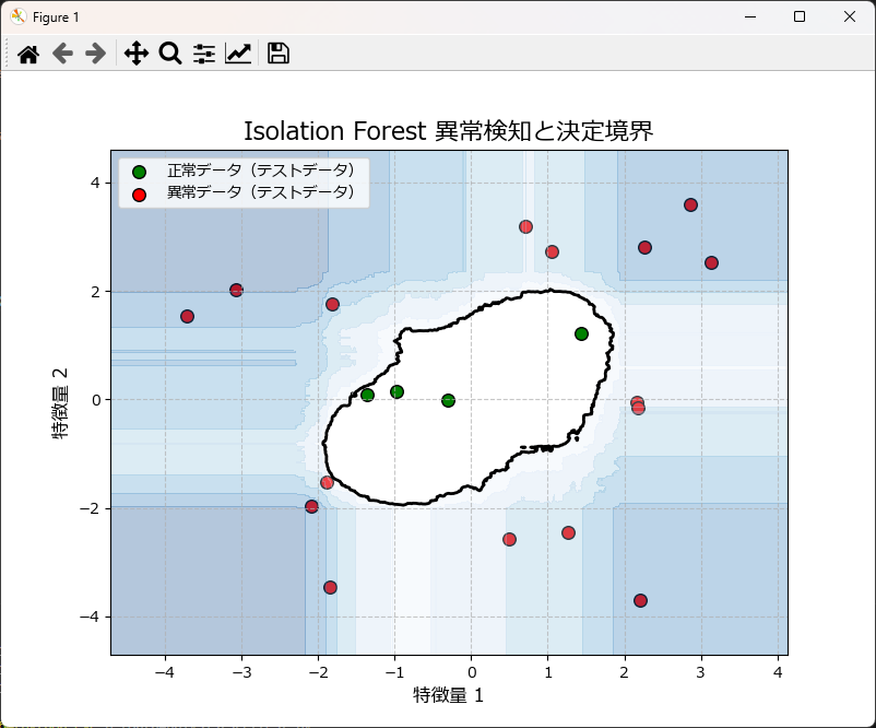
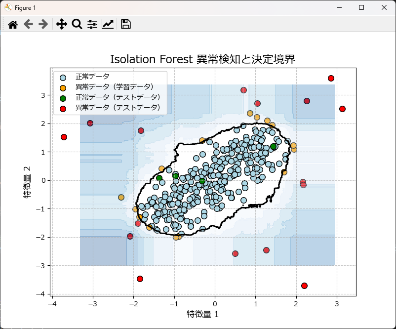
可視化
上記のグラフは、学習データ(正常)とテストデータ(異常)を散布図としてプロットし、さらに異常スコアで境界線(等高線)を描画したものです。
先ほどのプログラムの末尾に下記のコードを丸ごと挿入してもらえればグラフが描画されます。関数化しているので、コピペしてお使いいただけます。
import matplotlib.pyplot as plt
from matplotlib import rcParams
rcParams['font.family'] = 'Meiryo'

def plot_isolationforest_results(model, X_train=None, y_pred_train=None, X_test=None, y_pred_test=None):
    """
    2次元データのIsolation Forestの結果をプロットする。
    """
    plt.figure(figsize=(8, 6))

    if X_train is not None and y_pred_train is not None and X_train.ndim > 1:
        plt.scatter(X_train[y_pred_train == 1][:, 0], X_train[y_pred_train == 1][:, 1],
                    c='lightblue', edgecolors='k', s=70, label="正常データ")
        plt.scatter(X_train[y_pred_train == -1][:, 0], X_train[y_pred_train == -1][:, 1],
                    c='orange', edgecolors='k', s=70, label="異常データ(学習データ)")

    if X_test is not None and y_pred_test is not None and X_test.ndim > 1:
        plt.scatter(X_test[y_pred_test == 1][:, 0], X_test[y_pred_test == 1][:, 1],
                    c='green', edgecolors='k', s=70, label="正常データ(テストデータ)")
        plt.scatter(X_test[y_pred_test == -1][:, 0], X_test[y_pred_test == -1][:, 1],
                    c='red', edgecolors='k', s=70, label="異常データ(テストデータ)")

    xx, yy = np.meshgrid(np.linspace(X_train[:, 0].min() - 1, X_train[:, 0].max() + 1, 500),
                         np.linspace(X_train[:, 1].min() - 1, X_train[:, 1].max() + 1, 500))
    x_range = np.c_[xx.ravel(), yy.ravel()]

    Z = model.decision_function(x_range)
    Z = Z.reshape(xx.shape)

    plt.contour(xx, yy, Z, levels=[0], linewidths=2, colors='black')
    plt.contourf(xx, yy, Z, levels=np.linspace(Z.min(), 0, 7), cmap=plt.cm.Blues_r, alpha=0.3)

    plt.legend()
    plt.title("Isolation Forest 異常検知と決定境界", fontsize=16)
    plt.xlabel("特徴量 1", fontsize=12)
    plt.ylabel("特徴量 2", fontsize=12)
    plt.grid(True, linestyle='--', alpha=0.7)
    plt.show()

# プロット関数を実行
plot_isolationforest_results(model,X_train,y_pred_train,X_test,y_pred_test)
パラメータ調整とモデルの精度向上
Isolation Forestの主なパラメータには、次の項目があります。これらのパラメータを調整することで、モデルの精度を向上させることが可能です。特に、異常データの割合に応じて contamination を適切に設定することが重要です。
| パラメータ名 | 説明 | 調整のポイント |
|---|---|---|
| n_estimators | 決定木の数 | 多いほど精度向上に繋がるが、計算コストが増加。一般的に100~1000程度が使用される。 |
| max_samples | 各決定木を構築するためにサンプリングするデータの割合 | auto' (デフォルト): データセットのサイズに応じて自動的に決定。数値を指定することも可能。 |
| contamination | データセットにおける異常データの割合を推定するパラメータ | 異常データの割合を事前にある程度把握している場合に有効。 |
| max_features | 各決定木で分割に使用する特徴量の最大数を比率で指定 | 0~1の間で指定。 1:全ての特徴量を使用 0.5:特徴量の半分を使用 |
| random_state | 乱数生成器のシード | モデルの再現性を確保するために設定する。 |
predict() メソッドによる「1(正常)」「-1(異常)」の二値判定だけでなく、decision_function() で取得できる「異常スコア」も重要です。
閾値(contamination)を厳しくしすぎると誤検知が増え、緩すぎると異常を見逃します。まずはスコアの分布を可視化し、「異常の一歩手前」を捉えるための閾値を現場の感覚と照らし合わせて調整するのが運用のコツです。
ハイパーパラメータの調整には、クロスバリデーションを活用するのが効果的です。例えば、GridSerchCV を用いて最適なパラメータを探索できます。
from sklearn.ensemble import IsolationForest
from sklearn.model_selection import GridSearchCV

# ハイパーパラメータの探索範囲を設定
param_grid = {
    'contamination': [0.01, 0.05, 0.1],
    'n_estimators': [100, 200, 300],
    'max_samples': ['auto', 0.5, 1.0],
    'max_features': [1.0,0.5,0.1]
}

# GridSearchCVのインスタンスを作成
grid_search = GridSearchCV(IsolationForest(), param_grid, cv=5)

# グリッドサーチを実行
grid_search.fit(X_train)

# 最適なパラメータを表示
print("Best parameters:", grid_search.best_params_)ハイパーパラメータを調整しても異常検知の結果に満足できない場合は、特徴量エンジニアリングやデータの見直しを行います。
- 特徴量エンジニアリングの工夫(製造現場の知恵)
製造装置のデータは時系列であることが多いため、単なる「瞬間の値」だけでなく、以下の演算結果を特徴量として追加すると、iForestは「パターンの変化」を捉えやすくなります。- 移動平均・移動分散: ノイズを除去し、値の「揺らぎ」の異常を検知しやすくします。
- 変化率(デファレンス): 急激な上昇や下降を強調します。
- ラグ変数: 「10秒前の値」などを列として追加し、時間的な前後関係をモデルに教えます。
- スケーリングの特性について
Isolation Forestは決定木ベースのアルゴリズムであるため、距離ベースの手法(k-NNやSVM)とは異なり、特徴量ごとのスケールを揃える標準化(StandardScaler)を行わなくても動作するという強みがあります。ただし、分布が極端に偏っている場合は、対数変換などで分布を整えることが有効な場合もあります。 - 「異常スコア」の確認
判定が「1(正常)」か「-1(異常)」かで安定しない場合は、decision_function()を使って異常スコア(連続値)の分布を確認してください。閾値(contamination)を機械的に決めるのではなく、スコアのヒストグラムを見て「現場の違和感」と一致するポイントに境界線を引くのが運用のコツです。 - 別のアルゴリズムへの切り替え
データの特性によっては、以下の手法がより適している場合があります。- OneClassSVM: データが正規分布に近く、境界線をより厳密に引きたい場合。
- Local Outlier Factor (LOF): データの密度にムラがあり、局所的な外れ値を見つけたい場合。
- AutoEncoder(ディープラーニング): 高次元で複雑な非線形関係を持つデータの場合。
Isolation Forestが簡単に使える自作クラス
Isolation Forestを簡単に使えるようにするために自作クラスとグラフ描画関数を作成しました。
このクラスのfit() メソッドは、1次元データが渡された場合、内部でreshape(-1, 1)で2次元に拡張しているため、問題なく処理できます。
モデルを作成するには
IsolationForestUtilクラスのインスタンス生成時、引数にデータを格納したDataFrameを渡します。そして、fit メソッドにモデル作成で使いたいカラム名と、ハイパーパラメータを指定します。
read_csvメソッドを使うと、CSVファイルを読み込んでインスタンス変数(self.df)に保持します。
完成したモデルは save_modelメソッドで pickle ファイルとして保存できます。
# ~~~~~~~~~~~~~~~~~~~~~~~~~~~~~~~~~~~~~~~~~~~~~~~
# ここにIsolationForestUtilとグラフ描画関数のコードを張り付けるか、インポートしてください
# ~~~~~~~~~~~~~~~~~~~~~~~~~~~~~~~~~~~~~~~~~~~~~~~

# 学習データの生成
np.random.seed(42)
X_train_data = 0.5 * np.random.randn(100, 2)
X_train_data = np.r_[X_train_data + 1, X_train_data - 1, X_train_data]
df_train = pd.DataFrame(X_train_data, columns=['feature1', 'feature2'])

# インスタンスを生成
iso_for = IsolationForestUtil(df_train)

# モデルを学習
iso_for.fit(['feature1', 'feature2'], contamination=0.05, random_state=42)

# 学習データで異常検知を実施
y_pred_train = iso_for.predict(['feature1', 'feature2'])
print("Train predictions:", y_pred_train)

# モデルの保存
iso_for.save_model('isolation_forest_model.pkl')

# グラフ描画
plot_isolationforest_results(iso_for.model,X_train=df_train[['feature1', 'feature2']].values, y_pred_train=y_pred_train)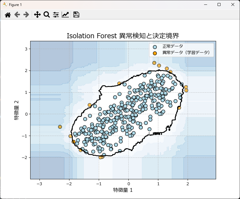
新しいデータで異常検知するには
IsolationForestUtilのインスタンス生成時にモデルファイルのパスを指定します。load_modelメソッドで後からモデルファイルを読み込むことも可能です。
predictメソッドにカラムを指定し、df引数にDataFrameを指定することで、新たなデータで異常検知が行えます。
# ~~~~~~~~~~~~~~~~~~~~~~~~~~~~~~~~~~~~~~~~~~~~~~~
# ここにIsolationForestUtilとグラフ描画関数のコードを張り付けるか、インポートしてください
# ~~~~~~~~~~~~~~~~~~~~~~~~~~~~~~~~~~~~~~~~~~~~~~~

# 学習データの生成
np.random.seed(42)
X_train_data = 0.5 * np.random.randn(100, 2)
X_train_data = np.r_[X_train_data + 1, X_train_data - 1, X_train_data]
df_train = pd.DataFrame(X_train_data, columns=['feature1', 'feature2'])

# インスタンスを生成
iso_for = IsolationForestUtil(df_train)

# モデルを学習
iso_for.fit(['feature1', 'feature2'], contamination=0.05, random_state=42)

# 学習データで異常検知を実施
y_pred_train = iso_for.predict(['feature1', 'feature2'])
print("Train predictions:", y_pred_train)

# テストデータを生成
np.random.seed(20)
X_test_data = np.random.uniform(low=-4, high=4, size=(20, 2))
df_test = pd.DataFrame(X_test_data, columns=['feature1', 'feature2'])

# テストデータで異常検知を実施
y_pred_test = iso_for.predict(['feature1', 'feature2'],df=df_test)
print("Test predictions:", y_pred_test)

# 学習データとテストデータの検知結果を合わせてグラフ描画
plot_isolationforest_results(iso_for.model,df_train[['feature1', 'feature2']].values, y_pred_train,df_test[['feature1', 'feature2']].values, y_pred_test)
モデル作成時にテストデータによる評価を行うには
基本的には前述の処理を続けて行えばよいのですが、少しだけ処理を簡素化しています。
# ~~~~~~~~~~~~~~~~~~~~~~~~~~~~~~~~~~~~~~~~~~~~~~~
# ここにIsolationForestUtilとグラフ描画関数のコードを張り付けるか、インポートしてください
# ~~~~~~~~~~~~~~~~~~~~~~~~~~~~~~~~~~~~~~~~~~~~~~~

# 学習データの生成
np.random.seed(42)
X_train_data = 0.5 * np.random.randn(100, 2)
X_train_data = np.r_[X_train_data + 1, X_train_data - 1, X_train_data]
df_train = pd.DataFrame(X_train_data, columns=['feature1', 'feature2'])

# インスタンスを生成
iso_for = IsolationForestUtil(df_train)

# モデルを学習
iso_for.fit(['feature1', 'feature2'], contamination=0.05, random_state=42)

# 学習データで異常検知を実施
y_pred_train = iso_for.predict(['feature1', 'feature2'])
print("Train predictions:", y_pred_train)

# テストデータを生成
np.random.seed(20)
X_test_data = np.random.uniform(low=-4, high=4, size=(20, 2))
df_test = pd.DataFrame(X_test_data, columns=['feature1', 'feature2'])

# テストデータで異常検知を実施
y_pred_test = iso_for.predict(['feature1', 'feature2'],df=df_test)
print("Test predictions:", y_pred_test)

# 学習データとテストデータの検知結果を合わせてグラフ描画
plot_isolationforest_results(iso_for.model,df_train[['feature1', 'feature2']].values, y_pred_train,df_test[['feature1', 'feature2']].values, y_pred_test)
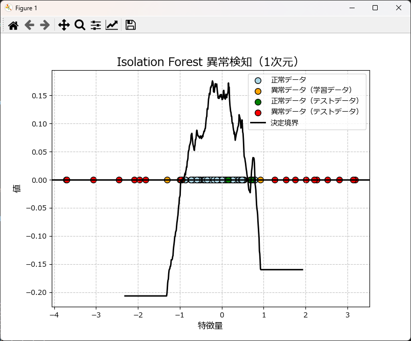
1次元の異常検知をするには
IsolationForestUtilクラスの使い方は前述と全く同じですが、グラフ描画は plot_ocsvm_results_1d を使用します。
# ~~~~~~~~~~~~~~~~~~~~~~~~~~~~~~~~~~~~~~~~~~~~~~~
# ここにIsolationForestUtilとグラフ描画関数のコードを張り付けるか、インポートしてください
# ~~~~~~~~~~~~~~~~~~~~~~~~~~~~~~~~~~~~~~~~~~~~~~~

# 学習データの生成
np.random.seed(42)
X_train_data = 0.5 * np.random.randn(100).reshape(-1, 1)
# 1次元データを2次元配列に変換
df_train = pd.DataFrame(X_train_data, columns=['feature1'])

# インスタンスを生成
iso_for = IsolationForestUtil(df_train)

# モデルを学習
iso_for.fit(['feature1'],contamination=0.05, random_state=42)

# 学習データで異常検知を実施
y_pred_train = iso_for.predict(['feature1'])
print("Train predictions:", y_pred_train)

# テストデータを生成
np.random.seed(20)
X_test_data = np.random.uniform(low=-4, high=4, size=(20,)).reshape(-1, 1)
df_test = pd.DataFrame(X_test_data, columns=['feature1'])

# テストデータで異常検知を実施
y_pred_test = iso_for.predict(['feature1'], df=df_test)
print("Test predictions:", y_pred_test)

# 1次元用の関数を使ってグラフ描画
plot_isolationforest_results_1d(
    iso_for.model,  # 学習したモデルを直接使用
    df_train[['feature1']].values,
    y_pred_train,
    df_test[['feature1']].values,
    y_pred_test
)
IsolationForestUtilクラスとグラフ描画関数リファレンス
| IsolationForestのグラフ描画関数 | 説明 |
|---|---|
| plot_isolationforest_results_1d( model, X_train=None, y_pred_train=None, X_test=None, y_pred_test=None ) | 1次元データのIsolationForestの結果をプロットする。学習データとテストデータを表示し、決定境界を描画する。 |
| plot_isolationforest_results( model, X_train=None, y_pred_train=None, X_test=None, y_pred_test=None ) | 2次元データのIsolationForestの結果をプロットする。学習データとテストデータを表示し、決定境界を描画する。 |
| IsolationForestUtilのメソッド | 説明 |
|---|---|
| __init__(df=None, model_path=None) | クラスの初期化メソッド。データフレームとモデルパスを受け取る。 |
| fit(column, nu=0.1, gamma="auto", kernel="rbf") | IsolationForestモデルを作成・学習するメソッド。指定したカラムを使用。 |
| predict(column, df=None) | 学習したモデルを使用して予測を行うメソッド。指定したカラムを使用。 |
| read_csv(file_name, encoding="shift-jis") | CSVファイルからデータを読み込むメソッド。 |
| save_model(model_path) | 学習したモデルをファイルに保存するメソッド。 |
| load_model(model_path=None) | モデルをファイルから読み込むメソッド。 |
IsolationForestUtilクラスとグラフ描画関数のソースコード
import numpy as np
import pandas as pd
from sklearn.ensemble import IsolationForest
import pickle
from sklearn.model_selection import GridSearchCV
import matplotlib.pyplot as plt
from matplotlib import rcParams
rcParams['font.family'] = 'Meiryo'

def plot_isolationforest_results_1d(model, X_train=None, y_pred_train=None, X_test=None, y_pred_test=None):
    """
    1次元データのIsolation Forestの結果をプロットする。

    学習データとテストデータを表示し、正常データと異常と検出されたデータを色分けしてプロットする。
    また、決定境界を描画する。

    Parameters:
    model : IsolationForestモデル
        学習済みのIsolationForestモデル。
    X_train : array-like, shape (n_samples,), optional
        学習データの特徴量。1次元データを想定。
    y_pred_train : array-like, shape (n_samples,), optional
        学習データに対する予測結果。1(正常)または-1(異常)。
    X_test : array-like, shape (n_samples,), optional
        テストデータの特徴量。1次元データを想定。
    y_pred_test : array-like, shape (n_samples,), optional
        テストデータに対する予測結果。1(正常)または-1(異常)。
    """
    plt.figure(figsize=(8, 6))

    # 学習データのプロット
    if X_train is not None and y_pred_train is not None:
        plt.scatter(X_train[y_pred_train == 1], np.zeros_like(X_train[y_pred_train == 1]),
                    c='lightblue', edgecolors='k', s=70, label="正常データ")
        plt.scatter(X_train[y_pred_train == -1], np.zeros_like(X_train[y_pred_train == -1]),
                    c='orange', edgecolors='k', s=70, label="異常データ(学習データ)")

    # テストデータのプロット
    if X_test is not None and y_pred_test is not None:
        plt.scatter(X_test[y_pred_test == 1], np.zeros_like(X_test[y_pred_test == 1]),
                    c='green', edgecolors='k', s=70, label="正常データ(テストデータ)")
        plt.scatter(X_test[y_pred_test == -1], np.zeros_like(X_test[y_pred_test == -1]),
                    c='red', edgecolors='k', s=70, label="異常データ(テストデータ)")

    plt.axhline(0, color='black', linewidth=2)

    # 決定境界を描画
    if X_train is not None or X_test is not None:
        x_range = np.linspace(X_train.min() - 1, X_train.max() + 1, 500).reshape(-1, 1) if X_train is not None else \
                  np.linspace(X_test.min() - 1, X_test.max() + 1, 500).reshape(-1, 1)

        Z = model.decision_function(x_range)
        plt.plot(x_range, Z, color='black', linewidth=2, label='決定境界')

    # グラフの設定
    plt.title("Isolation Forest 異常検知(1次元)", fontsize=16)
    plt.xlabel("特徴量", fontsize=12)
    plt.ylabel("値", fontsize=12)
    plt.grid(True, linestyle='--', alpha=0.7)
    plt.legend()
    plt.show()


def plot_isolationforest_results(model, X_train=None, y_pred_train=None, X_test=None, y_pred_test=None):
    """
    2次元データのIsolationForestの結果をプロットする。

    学習データとテストデータを表示し、正常データと異常と検出されたデータを色分けしてプロットする。
    また、決定境界を描画する。

    Parameters:
    model : IsolationForestモデル
        学習済みのIsolationForestモデル
    X_train : array-like, shape (n_samples, 2), optional
        学習データの特徴量。2次元データを想定。
    y_pred_train : array-like, shape (n_samples,), optional
        学習データに対する予測結果。1(正常)または-1(異常)。
    X_test : array-like, shape (n_samples, 2), optional
        テストデータの特徴量。2次元データを想定。
    y_pred_test : array-like, shape (n_samples,), optional
        テストデータに対する予測結果。1(正常)または-1(異常)。
    """
    plt.figure(figsize=(8, 6))

    # 学習データのプロット
    if X_train is not None and y_pred_train is not None and X_train.ndim > 1:
        plt.scatter(X_train[y_pred_train == 1][:, 0], X_train[y_pred_train == 1][:, 1],
                    c='lightblue', edgecolors='k', s=70, label="正常データ")
        plt.scatter(X_train[y_pred_train == -1][:, 0], X_train[y_pred_train == -1][:, 1],
                    c='orange', edgecolors='k', s=70, label="異常データ(学習データ)")

    # テストデータのプロット
    if X_test is not None and y_pred_test is not None and X_test.ndim > 1:
        plt.scatter(X_test[y_pred_test == 1][:, 0], X_test[y_pred_test == 1][:, 1],
                    c='green', edgecolors='k', s=70, label="正常データ(テストデータ)")
        plt.scatter(X_test[y_pred_test == -1][:, 0], X_test[y_pred_test == -1][:, 1],
                    c='red', edgecolors='k', s=70, label="異常データ(テストデータ)")

    # 決定境界の描画
    if X_train is not None and X_train.ndim > 1:
        xx, yy = np.meshgrid(np.linspace(X_train[:, 0].min() - 1, X_train[:, 0].max() + 1, 500),
                             np.linspace(X_train[:, 1].min() - 1, X_train[:, 1].max() + 1, 500))
        x_range = np.c_[xx.ravel(), yy.ravel()]

        Z = model.decision_function(x_range)
        Z = Z.reshape(xx.shape)

        plt.contour(xx, yy, Z, levels=[0], linewidths=2, colors='black')
        plt.contourf(xx, yy, Z, levels=np.linspace(Z.min(), 0, 7), cmap=plt.cm.Blues_r, alpha=0.3)
    elif X_test is not None and X_test.ndim > 1:
        xx, yy = np.meshgrid(np.linspace(X_test[:, 0].min() - 1, X_test[:, 0].max() + 1, 500),
                             np.linspace(X_test[:, 1].min() - 1, X_test[:, 1].max() + 1, 500))
        x_range = np.c_[xx.ravel(), yy.ravel()]

        Z = model.decision_function(x_range)
        Z = Z.reshape(xx.shape)

        plt.contour(xx, yy, Z, levels=[0], linewidths=2, colors='black')
        plt.contourf(xx, yy, Z, levels=np.linspace(Z.min(), 0, 7), cmap=plt.cm.Blues_r, alpha=0.3)

    plt.legend()
    plt.title("Isolation Forest 異常検知と決定境界", fontsize=16)
    plt.xlabel("特徴量 1", fontsize=12)
    plt.ylabel("特徴量 2", fontsize=12)
    plt.grid(True, linestyle='--', alpha=0.7)
    plt.show()

class IsolationForestUtil:
    def __init__(self, df=None, model_path=None):
        """
        IsolationForestModelクラスの初期化メソッド
        """
        self.df = None if df is None else df.copy()
        self.model = None if model_path is None else self.load_model(model_path)
        self.pred = []

    def fit(self, column, n_estimators=100, max_samples="auto",max_features=1.0,contamination="auto", random_state=None):
        """
        Isolation Forestモデルの作成と学習
        """

        # 指定されたカラムのデータを抽出
        if isinstance(column, list) and len(column) > 1:
            X = self.df[column].values
        else:
            X = self.df[column].values.reshape(-1, 1)  # 複数カラムのデータを2次元配列に変換

        self.model = IsolationForest(n_estimators=n_estimators, max_samples=max_samples,max_features=max_features,
                                     contamination=contamination, random_state=random_state).fit(X)
        return self.model

    def predict(self, column, df=None):
        """
        学習したモデルを使用して予測を行う
        """
        if df is not None:
            self.df = df

        # 指定されたカラムのデータを抽出
        if isinstance(column, list) and len(column) > 1:
            X = self.df[column].values
        else:
            X = self.df[column].values.reshape(-1, 1)  # 複数カラムのデータを2次元配列に変換

        self.pred = self.model.predict(X)
        return self.pred

    def read_csv(self, file_name, encoding="shift-jis"):
        self.df = pd.read_csv(file_name, encoding=encoding)

    def save_model(self, model_path):
        self.model_path = model_path
        with open(model_path, 'wb') as f:
            pickle.dump(self.model, f)

    def load_model(self, model_path=None):
        model_path = model_path if model_path else self.model_path
        with open(model_path, 'rb') as f:
            self.model = pickle.load(f)
        return self.model
まとめ
Isolation Forestは、異常検知に非常に効果的なアルゴリズムであり、特に製造業において設備や品質管理の自動化で活用されています。
高速かつ高精度な異常検知が可能なため、多くの企業で導入が進んでいます。
この記事が、皆さんの異常検知に役立てていただければ幸いです。


コメント