
製造業の現場では、データ分析やAIモデルの導入が進む中で、「どうやってモデルの性能を最大限に引き出すか」が重要な課題となっています。
その鍵を握るのが ハイパーパラメータの最適化。最適なハイパーパラメータを見つけることで、モデルの精度が劇的に向上し、生産性や品質管理の精度を高めることができます。
本記事では、製造業で活用できる グリッドサーチ と ランダムサーチ の具体的な手法を解説し、効果的なパラメータチューニングのポイントをお伝えします。
パラメータチューニングの概要
ハイパーパラメータは、モデルの訓練前に設定する重要なパラメータであり、学習プロセスに直接影響を与えます。これらのパラメータは、機械学習モデルの性能に大きく影響します。例えば、決定木の深さや学習率などです。
ハイパーパラメータを適切に最適化することで、モデルの予測精度や汎化性能(新しいデータへの適応力)が向上します。最適なパラメータを見つけることは、モデルがトレーニングデータに過度に適応せず、新しいデータに対しても高い精度を維持できることを意味します。
しかし、ハイパーパラメータチューニングは難しく、多くの試行錯誤と計算リソースが必要です。そこで、効率的にチューニングを行うための手法が用意されています。
主なハイパーパラメータチューニング手法
ハイパーパラメータチューニングとして有名なものは以下の通りです。この中で、グリッドサーチ、ランダムサーチ、ベイズ最適化が最も多く使われています。
本記事では、上記3つについて詳しく紹介しますが、それ以外はWindows上でサポートされていない、又はモジュールのバージョンへの依存関係が高いことで動作しないケースが多いため、本記事では割愛しています。
- グリッドサーチ(Grid Search):
- 概要: ハイパーパラメータのすべての組み合わせを網羅的に探索します。
- 利点: 全ての組み合わせを試すため、最適なパラメータセットを見つけやすい。
- 欠点: 計算コストが高く、大規模データや多くのパラメータがある場合は非効率。
- ランダムサーチ(Random Search):
- 概要: 指定された範囲内でランダムにハイパーパラメータを選び、最適な組み合わせを探索します。
- 利点: 広範囲のパラメータ空間を効率的に探索できる。
- 欠点: 最適なパラメータを見つけられる保証はない。
- ベイズ最適化(Bayesian Optimization):
- 概要: 既知の情報を基に、次に探索するパラメータを効率的に選択する。
- 利点: サンプル数が少なくても高精度なパラメータを見つけやすい。
- 欠点: 内部処理が複雑なため、処理が非常に重い
- 進化的アルゴリズム(Evolutionary Algorithms):
- 概要: 遺伝的アルゴリズムのように、進化過程をシミュレートして最適なパラメータを見つける。
- 利点: グローバルな最適解を見つける可能性が高い。
- 欠点: 計算リソースが多く必要。
- ハイパーバンド(Hyperband):
- 概要: 多数のハイパーパラメータセットを効率的に評価する方法。
- 利点: リソース効率が高く、計算時間を大幅に短縮できる。
- 欠点: 他の手法に比べて、まだ研究段階である。(但し、近年は使用されるケースが増えている)
- 自動機械学習(AutoML)
- 概要: 複数の最適化アルゴリズムやモデルアーキテクチャを組み合わせて、最適な機械学習モデルを構築。
- 利点: リソース効率が高く、計算時間を大幅に短縮が可能。最適化の詳細な知識がなくてもOK。
- 欠点: 選ばれたモデルは、必ずしも解釈しやすい訳ではない。計算リソースが多く必要になる場合あり。
グリッドサーチ (Grid Search)
グリッドサーチは、指定されたパラメータ空間の全ての組み合わせを試して最適なハイパーパラメータを見つける手法です。探索範囲が広い場合、計算コストが高くなることがあります。
下記はxgboost を使ったグリッドサーチのサンプルです。実際に使う手法に応じて適宜書き換えてご利用下さい。
分類モデルでの使用例
from sklearn.model_selection import GridSearchCV
import xgboost as xgb
from sklearn.datasets import load_iris
from sklearn.model_selection import train_test_split
from sklearn.metrics import accuracy_score

# Step1.データの準備
data = load_iris()
X, y = data.data, data.target
X_train, X_test, y_train, y_test = train_test_split(X, y, test_size=0.2, random_state=42)

# Step2.探索したいハイパーパラメータと探索の範囲を定義
param_grid = {
    'learning_rate': [0.01, 0.1, 0.2],
    'max_depth': [3, 5, 7],
    'n_estimators': [100, 200]
}

# Step3.グリッドサーチの対象となるモデルを作成
model = xgb.XGBClassifier()

# Step4.グリッドサーチの設定(モデル、探索範囲、精度評価のスコアリング、データの分割数、スレッド数を指定)
grid_search = GridSearchCV(estimator=model, param_grid=param_grid, scoring='accuracy', cv=3, n_jobs=-1)

# Step5.グリッドサーチの実行(テストデータを指定して実行)
grid_search.fit(X_train, y_train)

# Step6.最適なハイパーパラメータの取得
best_params = grid_search.best_params_
print(f"Best parameters: {best_params}")

# Step7.最適なハイパーパラメータでのモデル評価
best_model = grid_search.best_estimator_
y_pred = best_model.predict(X_test)
accuracy = accuracy_score(y_test, y_pred)
print(f"Accuracy: {accuracy * 100:.2f}%")
Best parameters: {'learning_rate': 0.01, 'max_depth': 3, 'n_estimators': 200}
Accuracy: 100.00%
回帰モデルでの使用例
from sklearn.model_selection import GridSearchCV
import xgboost as xgb
from sklearn.datasets import fetch_california_housing
from sklearn.model_selection import train_test_split
from sklearn.metrics import mean_squared_error

# Step1.データの準備
data = fetch_california_housing()
X, y = data.data, data.target
X_train, X_test, y_train, y_test = train_test_split(X, y, test_size=0.2, random_state=42)

# Step2.探索したいハイパーパラメータと探索の範囲を定義
param_grid = {
    'learning_rate': [0.01, 0.1, 0.2],
    'max_depth': [3, 5, 7],
    'n_estimators': [100, 200]
}

# Step3.グリッドサーチの対象となるモデルを作成
model = xgb.XGBRegressor()

# Step4.グリッドサーチの設定(モデル、探索範囲、精度評価のスコアリング、データの分割数、スレッド数を指定)
grid_search = GridSearchCV(estimator=model, param_grid=param_grid, scoring='neg_mean_squared_error', cv=3, n_jobs=-1)

# Step5.グリッドサーチの実行(テストデータを指定して実行)
grid_search.fit(X_train, y_train)

# Step6.最適なハイパーパラメータの取得
best_params = grid_search.best_params_
print(f"Best parameters: {best_params}")

# Step7.最適なハイパーパラメータでのモデル評価
best_model = grid_search.best_estimator_
y_pred = best_model.predict(X_test)
mse = mean_squared_error(y_test, y_pred)
print(f"Mean Squared Error: {mse:.4f}")
Best parameters: {'learning_rate': 0.2, 'max_depth': 5, 'n_estimators': 200}
Mean Squared Error: 0.2099
グリッドサーチのパラメータ
分類、回帰とも共通ですが、scoring (モデルの評価基準)が異なります。分類は scoring='accuracy'
回帰はscoring='neg_mean_squared_error'を指定します。
| 引数 | 説明 | 使用例 |
|---|---|---|
| estimator | 学習に使用するモデル(分類器や回帰器) | RandomForestClassifier(), XGBClassifier() |
| param_grid | チューニングしたいハイパーパラメータの候補を含む辞書。各パラメータに対してリストを指定し、全ての組み合わせを試す。 | {'n_estimators': [50, 100, 200], 'max_depth': [3, 5, 10]} |
| scoring | モデルの評価基準を指定。例えば、分類問題では 'accuracy' や 'f1' などが選べる。 | 'accuracy', 'f1', 'roc_auc' |
| cv | 交差検証でデータを分ける数。cv=3 だと3分割交差検証を行う。 | 3 |
| n_jobs | 並列処理するスレッド数。-1 は全てのCPUコアを使用する。 | -1(全コア使用)、2(2つのスレッド) |
2. ランダムサーチ (Random Search)
ランダムサーチは、指定されたパラメータ空間からランダムにサンプリングしてハイパーパラメータを見つける手法です。グリッドサーチよりも計算コストが低く、探索範囲を広げやすいというメリットがあります。
下記はxgboost を使ったグリッドサーチのサンプルです。実際に使う手法に応じて適宜書き換えてご利用下さい。
分類モデルでの使用例
from sklearn.model_selection import RandomizedSearchCV
import xgboost as xgb
from sklearn.datasets import load_iris
from sklearn.model_selection import train_test_split
from sklearn.metrics import accuracy_score
import numpy as np

# データの準備
data = load_iris()
X, y = data.data, data.target
X_train, X_test, y_train, y_test = train_test_split(X, y, test_size=0.2, random_state=42)

# Step2.探索したいハイパーパラメータと探索の範囲を定義
param_dist = {
    'learning_rate': np.linspace(0.01, 0.2, 20),
    'max_depth': np.arange(3, 10),
    'n_estimators': np.arange(50, 300, 50)
}

# Step3.ランダムサーチの対象となるモデルを作成
model = xgb.XGBClassifier()

# Step4.ランダムサーチの設定(モデル、探索範囲、精度評価のスコアリング、データの分割数、スレッド数を指定)
random_search = RandomizedSearchCV(estimator=model, param_distributions=param_dist, n_iter=100, scoring='accuracy', cv=3, n_jobs=-1, random_state=42)

# Step5.ランダムサーチの実行(テストデータを指定して実行)
random_search.fit(X_train, y_train)

# Step6.最適なハイパーパラメータの取得
best_params = random_search.best_params_
print(f"Best parameters: {best_params}")

# Step7.最適なハイパーパラメータでのモデル評価
best_model = random_search.best_estimator_
y_pred = best_model.predict(X_test)
accuracy = accuracy_score(y_test, y_pred)
print(f"Accuracy: {accuracy * 100:.2f}%")
Best parameters: {'n_estimators': 50, 'max_depth': 6, 'learning_rate': 0.05}
Accuracy: 100.00%
回帰モデルでの使用例
from sklearn.model_selection import RandomizedSearchCV
import xgboost as xgb
from sklearn.datasets import fetch_california_housing
from sklearn.model_selection import train_test_split
from sklearn.metrics import mean_squared_error
import numpy as np

# データの準備
data = fetch_california_housing()
X, y = data.data, data.target
X_train, X_test, y_train, y_test = train_test_split(X, y, test_size=0.2, random_state=42)

# Step2.探索したいハイパーパラメータと探索の範囲を定義
param_dist = {
    'learning_rate': np.linspace(0.01, 0.2, 20),
    'max_depth': np.arange(3, 10),
    'n_estimators': np.arange(50, 300, 50)
}

# Step3.ランダムサーチの対象となるモデルを作成
model = xgb.XGBRegressor()

# Step4.ランダムサーチの設定(モデル、探索範囲、精度評価のスコアリング、データの分割数、スレッド数を指定)
random_search = RandomizedSearchCV(estimator=model, param_distributions=param_dist, n_iter=100, scoring='neg_mean_squared_error', cv=3, n_jobs=-1, random_state=42)

# Step5.ランダムサーチの実行(テストデータを指定して実行)
random_search.fit(X_train, y_train)

# Step6.最適なハイパーパラメータの取得
best_params = random_search.best_params_
print(f"Best parameters: {best_params}")

# Step7.最適なハイパーパラメータでのモデル評価
best_model = random_search.best_estimator_
y_pred = best_model.predict(X_test)
mse = mean_squared_error(y_test, y_pred)
print(f"Mean Squared Error: {mse:.4f}")
Best parameters: {'n_estimators': 250, 'max_depth': 7, 'learning_rate': 0.06999999999999999}
Mean Squared Error: 0.2086
ランダムサーチのパラメータ
| 引数 | 説明 | 使用例 |
|---|---|---|
| estimator | 学習に使用するモデル(分類器や回帰器) | RandomForestClassifier(), XGBClassifier() |
| param_distributions | チューニングしたいハイパーパラメータの候補を含む辞書。GridSearchCV の param_grid と異なり、リストだけでなく分布も指定できる。 | {'n_estimators': [50, 100, 200], 'max_depth': sp_randint(1, 10)} |
| n_iter | ランダムサーチで試すパラメータの組み合わせ数。GridSearchCV では全組み合わせを試しますが、ランダムサーチでは指定した回数だけ試します。 | 100(100回ランダムにパラメータを選んで試す) |
| scoring | モデルの評価基準を指定。GridSearchCV と同じ。 | 'accuracy', 'f1', 'roc_auc' |
| cv | 交差検証でデータを分ける数。cv=3 だと3分割交差検証を行う。 | 3 |
| n_jobs | 並列処理するスレッド数。-1 は全てのCPUコアを使用する。 | -1(全コア使用)、2(2つのスレッド) |
ベイズ最適化
ベイズ最適化は、効率的にハイパーパラメータを探索する手法で、特に高価な評価関数や計算リソースが限られている場合に有効です。基本的な考え方は、既存の情報を利用して次に試すべきパラメータの組み合わせを賢く選ぶことです。
実装ライブラリとしては、Python 製の Optuna が代表的です。Optuna はデフォルトで TPE(Tree-structured Parzen Estimator)というベイズ最適化アルゴリズムを採用しており、少ない試行回数でも高精度な結果が得られやすいのが特徴です。さらに、早期終了(pruning)や可視化機能も備えており、実務でも広く使われています。
分類モデルでの使用例
import optuna
from sklearn.ensemble import RandomForestClassifier
from sklearn.model_selection import cross_val_score
from sklearn.datasets import make_classification
from sklearn.model_selection import train_test_split

# データ作成
X, y = make_classification(n_samples=1000, n_features=20, n_informative=10, n_redundant=10, random_state=42)
X_train, X_test, y_train, y_test = train_test_split(X, y, test_size=0.2, random_state=42)

# 目的関数
def objective(trial):
    # ハイパーパラメータの探索範囲
    param = {
        'n_estimators': trial.suggest_int('n_estimators', 10, 200),
        'max_depth': trial.suggest_int('max_depth', 3, 20),
        'min_samples_split': trial.suggest_int('min_samples_split', 2, 10),
        'min_samples_leaf': trial.suggest_int('min_samples_leaf', 1, 10),
    }

    model = RandomForestClassifier(**param)
    score = cross_val_score(model, X_train, y_train, cv=3, scoring='accuracy').mean()
    return score

# 最適化
study = optuna.create_study(direction='maximize')
study.optimize(objective, n_trials=50)

# 最適なパラメータと結果
print("Best parameters:", study.best_params)
print("Best score:", study.best_value)
[I 2024-12-01 15:38:57,233] Trial 47 finished with value: 0.9075028394957432 and parameters: {'n_estimators': 164, 'max_depth': 18, 'min_samples_split': 6, 'min_samples_leaf': 1}. Best is trial 41 with value: 0.9087371988022491.
[I 2024-12-01 15:38:57,803] Trial 48 finished with value: 0.9062450132822694 and parameters: {'n_estimators': 136, 'max_depth': 18, 'min_samples_split': 6, 'min_samples_leaf': 1}. Best is trial 41 with value: 0.9087371988022491.
[I 2024-12-01 15:38:58,366] Trial 49 finished with value: 0.8999934292660491 and parameters: {'n_estimators': 133, 'max_depth': 18, 'min_samples_split': 6, 'min_samples_leaf': 1}. Best is trial 41 with value: 0.9087371988022491.
Best parameters: {'n_estimators': 189, 'max_depth': 18, 'min_samples_split': 5, 'min_samples_leaf': 2}
Best score: 0.9087371988022491
回帰モデルでの使用例
import optuna
from sklearn.ensemble import RandomForestRegressor
from sklearn.model_selection import cross_val_score
from sklearn.datasets import fetch_california_housing
from sklearn.model_selection import train_test_split

# データ作成
data = fetch_california_housing()
X, y = data.data, data.target
X_train, X_test, y_train, y_test = train_test_split(X, y, test_size=0.2, random_state=42)

# 目的関数
def objective(trial):
    # ハイパーパラメータの探索範囲
    param = {
        'n_estimators': trial.suggest_int('n_estimators', 10, 200),
        'max_depth': trial.suggest_int('max_depth', 3, 20),
        'min_samples_split': trial.suggest_int('min_samples_split', 2, 10),
        'min_samples_leaf': trial.suggest_int('min_samples_leaf', 1, 10),
    }

    model = RandomForestRegressor(**param)
    score = cross_val_score(model, X_train, y_train, cv=3, scoring='neg_mean_squared_error').mean()
    return score

# 最適化
study = optuna.create_study(direction='maximize')
study.optimize(objective, n_trials=50)

# 最適なパラメータと結果
print("Best parameters:", study.best_params)
print("Best score:", -study.best_value)
[I 2024-12-01 16:19:35,869] Trial 47 finished with value: -0.2656001997309059 and parameters: {'n_estimators': 183, 'max_depth': 18, 'min_samples_split': 5, 'min_samples_leaf': 1}. Best is trial 21 with value: -0.26388663557893227.
[I 2024-12-01 16:19:43,991] Trial 48 finished with value: -0.27205338958691255 and parameters: {'n_estimators': 54, 'max_depth': 20, 'min_samples_split': 4, 'min_samples_leaf': 4}. Best is trial 21 with value: -0.26388663557893227.
[I 2024-12-01 16:20:13,495] Trial 49 finished with value: -0.26731512868779844 and parameters: {'n_estimators': 191, 'max_depth': 17, 'min_samples_split': 7, 'min_samples_leaf': 3}. Best is trial 21 with value: -0.26388663557893227.
Best parameters: {'n_estimators': 196, 'max_depth': 20, 'min_samples_split': 5, 'min_samples_leaf': 2}
Best score: 0.26388663557893227
ベイズ最適化のパラメータ
create_study で指定できるパラメータ一覧
| パラメータ | 説明 | デフォルト値 |
|---|---|---|
| study_name | Studyの名前。データベースの識別子として使用されます。 | None |
| storage | Studyの状態を保存するためのストレージ(例:SQLite URL)。 | None |
| sampler | ハイパーパラメータのサンプリング方法(例:TPESampler)。 | TPESampler |
| pruner | 早期終了のためのプルーナー(例:MedianPruner)。 | None |
| direction | 最適化の方向('minimize' または 'maximize')。 | 'minimize' |
| load_if_exists | Studyが既に存在する場合にロードするかどうか。 | False |
| directions | 多目的最適化のための最適化方向のリスト。 | None |
| study_id | 特定のIDを持つStudyを作成またはロードします。 | None |
optimize で指定できるパラメータ一覧
| パラメータ | 説明 | デフォルト値 |
|---|---|---|
| func | 最適化する目的関数。 | なし(必須) |
| n_trials | 最適化の試行回数。 | None |
| timeout | 最適化を実行する最大時間(秒数)。 | None |
| n_jobs | 並列に実行する試行の数。 | 1 |
| catch | キャッチする例外のクラスまたはタプル。 | (Exception,) |
| callbacks | 各試行後に呼び出されるコールバック関数のリスト。 | None |
| gc_after_trial | 各試行の後にガベージコレクションを実行するかどうか。 | False |
| show_progress_bar | 進行状況バーを表示するかどうか。 | False |
ラメータチューニングの自作クラス
sklearnで用意されている iris_data を使って、パラメータチューニング自作クラスの使い方を説明します。
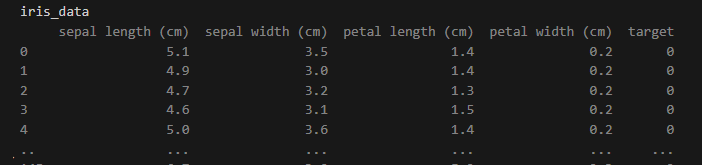
- データセットをDataFrameに読み込む。
- ハイパーパラメータの範囲を param_dist にセットする。
- チューニング対象の分類器(モデル)を作成する。
- HyperparameterTuningに、モデル、ハイパーパラメータの範囲、DataFrame、目的変数のカラム、特徴量のカラムを指定してインスタンスを生成する。
- サーチ方法に応じたメソッド(grid_search()、random_search()、bayes_search())を呼び出す。
# 使用例(分類)
iris_data = load_iris(as_frame=True).frame
feature_columns = iris_data.columns[:-1].tolist() # 特徴量のカラム名のリストを取得
target_column = iris_data.columns[-1] # 目的変数のカラム名を取得
param_dist = {
    'n_estimators': [100, 200, 300],
    'max_depth': [None, 10, 20, 30],
    'min_samples_split': [2, 5, 10],
    'min_samples_leaf': [1, 2, 4],
    'bootstrap': [True, False]
}
model = RandomForestClassifier(random_state=42)

tuner = HyperparameterTuning(model, param_dist, iris_data, feature_columns, target_column)
tuner.grid_search()  # グリッドサーチを実行
Best parameters: {'bootstrap': True, 'max_depth': None, 'min_samples_leaf': 2, 'min_samples_split': 2, 'n_estimators': 100}
Accuracy: 100.00%
リファレンス
| メソッド名 | 説明 | パラメータ | 戻り値 |
|---|---|---|---|
| init | クラスの初期化 | model: 調整する機械学習モデル param_dist: ハイパーパラメータ探索範囲 data: データセット feature_columns: 特徴量のカラム名リスト target_column: 目標変数のカラム名 | なし |
| _print_results | 最適なハイパーパラメータとモデルの評価結果を出力 | best_params: 最適なハイパーパラメータ best_model: 最適なハイパーパラメータで訓練されたモデル | なし |
| grid_search | グリッドサーチを使用してハイパーパラメータの最適化を行います。 | なし | なし |
| random_search | ランダムサーチを使用してハイパーパラメータの最適化を行います。 | なし | なし |
| bayes_search | ベイズ最適化を使用してハイパーパラメータの最適化を行います。 | なし | なし |
自作クラスのソースコード
import optuna
from sklearn.model_selection import GridSearchCV, RandomizedSearchCV, train_test_split, cross_val_score
from sklearn.metrics import accuracy_score, mean_squared_error

class HyperparameterTuning:
    """
    ハイパーパラメータチューニングを行うクラス。
    渡されたモデルとハイパーパラメータの範囲を用いて、グリッドサーチ、ランダムサーチ、ベイズ最適化を行います。

    Attributes:
        model (estimator): 調整する機械学習モデル。
        param_dist (dict): ハイパーパラメータの探索範囲。
        X_train (DataFrame): トレーニングデータの特徴量。
        X_test (DataFrame): テストデータの特徴量。
        y_train (Series): トレーニングデータのラベル。
        y_test (Series): テストデータのラベル。
        is_classification (bool): モデルが分類器かどうかを示すフラグ。
    """

    def __init__(self, model, param_dist, data, feature_columns, target_column):
        """
        コンストラクタ。モデル、ハイパーパラメータの範囲、およびデータを初期化します。

        Args:
            model (estimator): 調整する機械学習モデル。
            param_dist (dict): ハイパーパラメータの探索範囲。
            data (DataFrame): データセット。
            feature_columns (list): 特徴量のカラム名リスト。
            target_column (str): 目標変数のカラム名。
        """
        self.model = model
        self.param_dist = param_dist
        self.X = data[feature_columns]
        self.y = data[target_column]
        self.X_train, self.X_test, self.y_train, self.y_test = train_test_split(self.X, self.y, test_size=0.2, random_state=42)
        self.is_classification = hasattr(model, "predict_proba")

    def _print_results(self, best_params, best_model):
        """
        最適なハイパーパラメータとモデルの評価結果を出力します。

        Args:
            best_params (dict): 最適なハイパーパラメータ。
            best_model (estimator): 最適なハイパーパラメータで訓練されたモデル。
        """
        print(f"Best parameters: {best_params}")
        y_pred = best_model.predict(self.X_test)
        if self.is_classification:
            accuracy = accuracy_score(self.y_test, y_pred)
            print(f"Accuracy: {accuracy * 100:.2f}%")
        else:
            mse = mean_squared_error(self.y_test, y_pred)
            print(f"Mean Squared Error: {mse:.4f}")

    def grid_search(self):
        """
        グリッドサーチを使用してハイパーパラメータの最適化を行います。
        """
        search = GridSearchCV(estimator=self.model, param_grid=self.param_dist, scoring='accuracy' if self.is_classification else 'neg_mean_squared_error', cv=3, n_jobs=-1)
        search.fit(self.X_train, self.y_train)
        self._print_results(search.best_params_, search.best_estimator_)

    def random_search(self):
        """
        ランダムサーチを使用してハイパーパラメータの最適化を行います。
        """
        search = RandomizedSearchCV(estimator=self.model, param_distributions=self.param_dist, n_iter=100, scoring='accuracy' if self.is_classification else 'neg_mean_squared_error', cv=3, n_jobs=-1, random_state=42)
        search.fit(self.X_train, self.y_train)
        self._print_results(search.best_params_, search.best_estimator_)

    def bayes_search(self):
        """
        ベイズ最適化を使用してハイパーパラメータの最適化を行います。
        """
        def objective(trial):
            """
            ベイズ最適化の目的関数。ハイパーパラメータを提案し、モデルの評価スコアを返します。

            Args:
                trial (Trial): Optunaのトライアルオブジェクト。

            Returns:
                float: モデルの評価スコア。
            """
            params = {}
            for key, value in self.param_dist.items():
                if isinstance(value, list):
                    params[key] = trial.suggest_categorical(key, value)
                elif isinstance(value, tuple):
                    params[key] = trial.suggest_uniform(key, *value)
                elif isinstance(value, range):
                    params[key] = trial.suggest_int(key, value.start, value.stop - 1)
            model = self.model.__class__(**params)
            score = cross_val_score(model, self.X_train, self.y_train, cv=3, scoring='accuracy' if self.is_classification else 'neg_mean_squared_error').mean()
            return score

        study = optuna.create_study(direction='maximize' if self.is_classification else 'minimize')
        study.optimize(objective, n_trials=50)
        self._print_results(study.best_params, self.model.__class__(**study.best_params))
まとめ
ハイパーパラメータチューニングは、機械学習モデルの性能を最大化する重要な作業です。
本記事では、グリッドサーチ、ランダムサーチ、ベイズ最適化という3つの手法を紹介しました。
グリッドサーチ
- 最適解を見つける精度が高いが、計算コストが非常に高い。
- 探索範囲が狭い場合に適している。
ランダムサーチ
- 効率よく探索でき、計算コストが比較的低い。
- 最適解を見逃す可能性があるが、探索範囲が広い場合に有効。
ベイズ最適化
- 理論上は効率的だが、計算コストが高く感じられることがある。
- 探索過程を賢く進め、少ない試行回数で最適解に近づくことを目指す。
また、この3つの手法を簡単に利用するための自作クラスについても、使い方とプログラムコードを紹介しました。
本記事を参考に、是非ハイパーパラメータチューニングにトライしてみてください。


コメント