
画像認識技術は、AI やコンピュータビジョンの進化とともに急速に発展しています。その中でも、SIFT (Scale-Invariant Feature Transform) は、スケールや回転変化に強い特徴点検出手法として注目されています。
本記事では、Python と OpenCV を活用し、SIFT を使った 特徴量ベースの画像分類手法 を紹介します。
サンプルデータやサンプルコードを用いて、SIFT の仕組みと具体的な使い方を分かり易く解説していますので、興味のある方は、是非ご一読ください。
SIFTとは?
SIFT(Scale-Invariant Feature Transform、スケール不変特徴変換)は、画像内の特徴点(キーポイント)を抽出し、それらを記述するためのアルゴリズムで、主に物体認識や画像マッチング、3D再構成などに広く使われています。2004年にDavid Loweによって提案されました。
SIFTは一時期特許がありましたが、2020年に期限が切れ、現在は商用でも使用可能(OpenCV 4.4以降)です。
SIFTによって抽出された特徴量を、どのように利用するかによって、画像分類やオブジェクト検出、画像検索など、様々な用途に活用できます。
SIFTの活用例
- 画像分類 → 類似した特徴点をクラスタリングし、画像カテゴリを判別
- オブジェクト検出 → 特定のパターン(印鑑やロゴなど)が画像のどこにあるか探す
- 画像検索 → データベース内の画像から一致する特徴を持つものを検索
- 偽造防止 → 印影やサインの真正性を特徴点ベースで確認
- AR(拡張現実) → 現実の物体を特徴点で認識し、バーチャル情報を重ねる
SIFTの特徴
- スケール不変性:画像の大きさが変わっても検出される特徴点は同じ
- 回転不変性:画像が回転しても対応する特徴点が検出される
- 照明変化に強い:局所的な輝度変化やコントラスト変化に耐性がある
- 部分的な遮蔽にも強い:一部が隠れていても対応点を見つけられる
- 計算コストが高い:リアルタイム処理には不向きな場合がある
| 特徴量 | スケール不変 | 回転不変 | 処理速度 | 精度 |
|---|---|---|---|---|
| SIFT | ◎ | ◎ | △(遅め) | ◎ |
| SURF | ◎ | ◎ | ○ | ○ |
| ORB | △ | ◎ | ◎(速い) | △ |
SIFTの処理ステップ
- スケール空間の構築
画像を異なるサイズ(解像度)に変換。
各スケールでガウシアンフィルターを適用し、滑らかにする。
DoG(Difference of Gaussian)を使って、輪郭や特徴的な部分を強調。 - 特徴点の検出(極値探索)
スケール空間の中で、周囲より明るい or 暗い点(極値)を探す。
これが「特徴点候補」となる。 - 特徴点の精査(ノイズ除去)
エッジやノイズによる誤検出を防ぐため、信頼性の低い特徴点を削除。
例えば、直線的なエッジは特徴として弱いため除外する。 - 主方向の割り当て(回転への対応)
各特徴点に主要な向き(オリエンテーション)を設定。
画像が回転しても同じ特徴点として認識できるようになる。 - 特徴記述子の作成(データ化)
特徴点の周囲のピクセルの勾配情報を計算。
128次元のベクトルとして記録し、他の画像と比較できるようにする。
SIFTの基本的な使い方
ターゲット画像
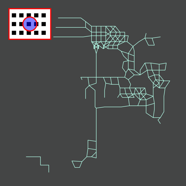
特徴量抽出結果
上図は、今回の分類に用いるターゲット画像(左側)と、SIFTで得られた特徴量の結果(右側)を並べたものです。
そして、下記はそのサンプルプログラムです。
試したい場合は、ターゲット画像を右クリックでダウンロードし、パスをご自身の環境に書き換えて実行してください。
import cv2
import numpy as np

# 画像を読み込む
image = cv2.imread(r"P:\target.png", cv2.IMREAD_GRAYSCALE)

# SIFTの特徴抽出器を作成
sift = cv2.SIFT_create()

# キーポイントと特徴量を抽出
keypoints, descriptors = sift.detectAndCompute(image, None)

# キーポイントを画像に描画
image_with_keypoints = cv2.drawKeypoints(image, keypoints, None)

# 画像を表示
cv2.imshow("SIFT Keypoints", image_with_keypoints)
cv2.waitKey(0)
cv2.destroyAllWindows()
SIFTを活用した画像検索
では、さっそく試してみましょう。
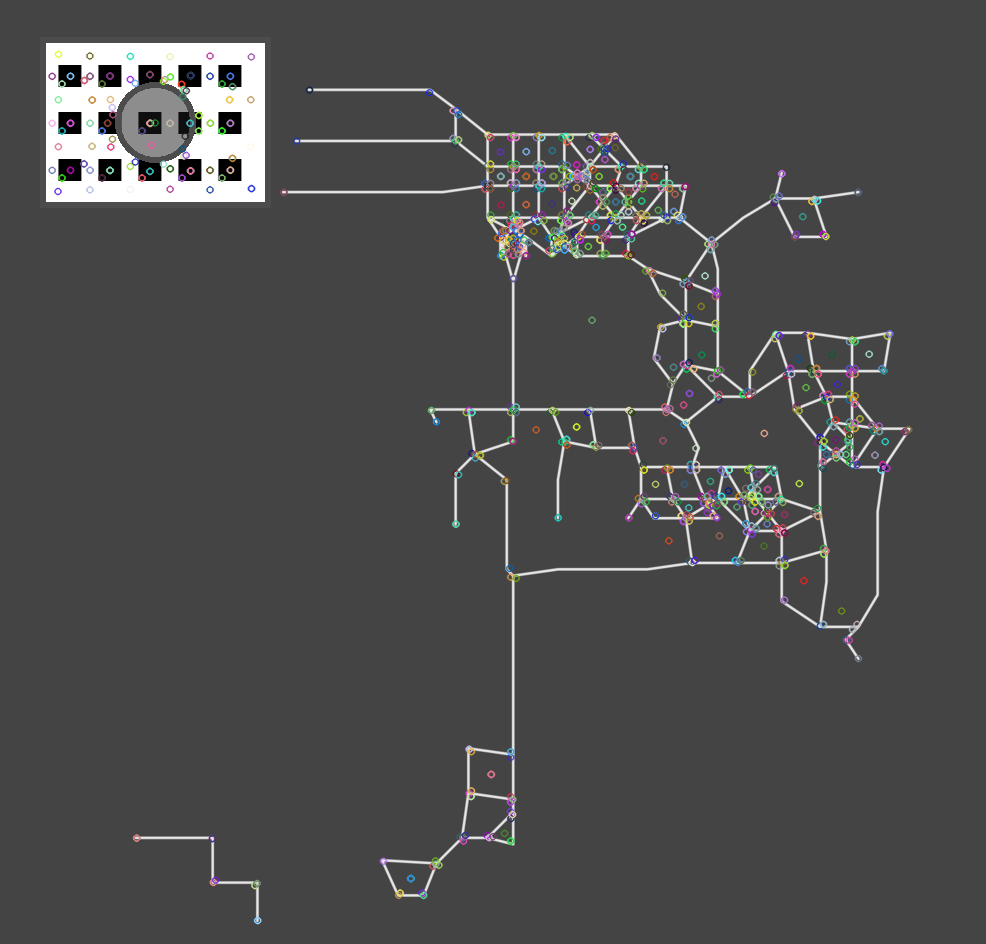
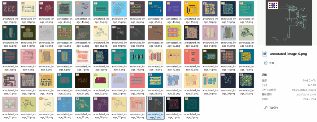
下記のプログラムは、前章で紹介した annotated_image_0.png と類似する画像を、サンプル画像から探すものです。cv2.BFMatcher(最近傍探索)に抽出した特徴量と、判定したい画像を渡すことで、類似度を算出しています。
尚、類似度は小さいほど類似性が高く、数値が大きくなるほど類似していないと判断します。
実験したい場合は、5行目をご自身の環境に合わせて書き換えてから実行してください。
import cv2
import os

# 特徴画像の読み込み(比較対象となる基準画像)
target_img = cv2.imread(r"P:\target.png", cv2.IMREAD_GRAYSCALE)

# SIFT特徴抽出を行うためのオブジェクトを作成
sift = cv2.SIFT_create()

# 基準画像の特徴点と記述子(descriptors)を抽出
_, descriptors_target = sift.detectAndCompute(target_img, None)

# Brute Force Matcher(最近傍探索)を設定
# NORM_L2はSIFTのような浮動小数点の記述子と相性が良い
bf = cv2.BFMatcher(cv2.NORM_L2, crossCheck=True)

# 類似度を比較する画像が保存されているフォルダ(検索対象フォルダ)
search_folder = r"P:\annotated_images"

# 画像ファイルごとの類似度を記録するリスト
results = []

# フォルダ内の全画像を処理
for image_file in os.listdir(search_folder):

    # 画像ファイルのパスを取得し、グレースケールで読み込み
    image = cv2.imread(os.path.join(search_folder, image_file), cv2.IMREAD_GRAYSCALE)

    # 現在処理している画像の特徴点と記述子を抽出
    _, descriptors = sift.detectAndCompute(image, None)

    # 特徴点のマッチング(基準画像と現在の画像を比較)
    matches = bf.match(descriptors_target, descriptors)

    # マッチした特徴点の距離の平均を類似度スコアとして計算
    # 距離が小さいほど、画像同士が類似していると判断できる
    score = sum(m.distance for m in matches) / len(matches)

    # 画像ファイル名と類似度スコアを記録
    results.append((image_file, round(score, 2)))

# 類似度スコアを表示
for file, score in results:
    print(f"{file}: 類似度スコア {score}")
結果は次の通りです。annotated_image_0.png (ターゲット画像そのもの)の類似度は0(類似性が高い)と判定されました。
興味深いのは、それ以外の画像において、類似度のバラつきが存在する点です。
annotated_image_0.png: 類似度スコア 0.0
annotated_image_1.png: 類似度スコア 237.11
annotated_image_10.png: 類似度スコア 77.16
annotated_image_11.png: 類似度スコア 314.61
annotated_image_12.png: 類似度スコア 282.82
annotated_image_13.png: 類似度スコア 296.56
annotated_image_14.png: 類似度スコア 257.51
annotated_image_15.png: 類似度スコア 89.12
annotated_image_16.png: 類似度スコア 265.02
~~~~~以下省略~~~~~
下記のプログラムは、上記プログラムの出力結果 results を棒グラフ化するものです。プログラムでは、類似度が150以下のものは赤で表示しています。
import matplotlib.pyplot as plt
from matplotlib import rcParams
import re

rcParams['font.family'] = 'Meiryo'

# 連番でソート
results.sort(key=lambda x: int(re.search(r"_(\d+)", x[0]).group(1)))

# 連番とスコアをそれぞれのリストに格納
serial_numbers = [int(re.search(r"_(\d+)", file).group(1)) for file, score in results]
scores = [score for _, score in results]

# 縦棒グラフを作成
plt.figure(figsize=(10, 6))
plt.bar(serial_numbers, scores, color="skyblue")
plt.xlabel("画像の連番")
plt.ylabel("類似度スコア")
plt.title("画像の類似度スコア(連番順)")
plt.xticks(serial_numbers)
plt.grid(axis="y", linestyle="--", alpha=0.5)

# グラフを表示
plt.show()
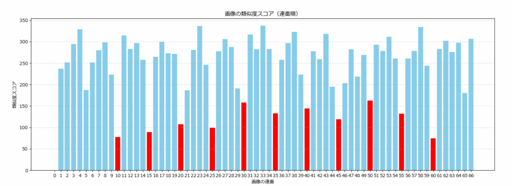
赤は全て、左上のマークが同一の画像です。annotated_image_5とannotated_image_65 の2枚のみ、150を超えてしまいましたが、それ以外は150未満(他に比べて類似性が高い)です。
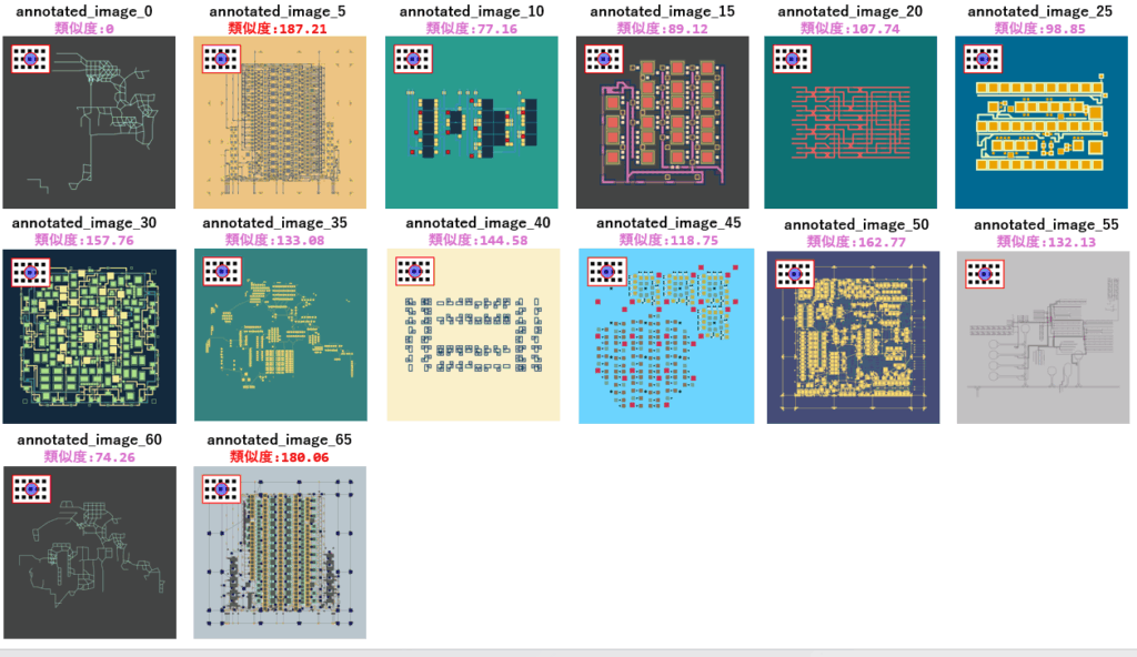
以上のことから、左上のマーク部分の特徴量も正しく抽出されており、類似度の計算においても反映されていることが分かります。
左上のマークだけを切り出して特徴量を求め、それを使ってサンプル画像から同じマークのある画像の分類を試みましたが、うまく分類できませんでした。これは、画像の解像度が小さいと、抽出される特徴量が少なくなるため、精度が低下します。リサイズ等で解像度を増やす等の対策が必要です。
SIFT+機械学習による画像分類
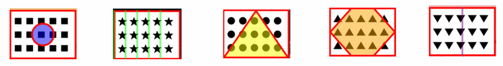
サンプル画像の左上には、5種類のマークが書き込まれていますので、SIFTと機械学習を組み合わせて画像分類してみましょう。
組み合わせる機械学習としては、クラスタリングやランダムフォレスト、SVNなどがよく使われますが、ここでは教師無し学習として、クラスタリングを使った方法を紹介します。
SIFT+クラスタリングによる画像分類
SIFTで得られた特徴量を、クラスタリング(K-meansやDBSCAN)を使って画像分類する方法がよく用いられます。
サンプルプログラムでは、次のステップで処理を進めています。
- 矩形領域の切り出し(背景画像の削除)
マークが描かれていると思われる、おおよその範囲を切り出します。 - 画像の拡大
解像度が少ないことで、特徴量が少なくなるのを避けるため、画像を3倍に拡大します。 - SIFT特徴抽出
各画像から特徴量を抽出します。 - K-meansクラスタリング
特徴量をK-meansで5つのクラスタに分類します。 - 画像整理
分類結果に基づき、画像を対応するクラスのフォルダにコピーします。
import cv2
import numpy as np
import os
import shutil
from sklearn.cluster import KMeans
def extract_sift_features(image_folder, crop_coords):
"""
指定フォルダ内の画像からSIFT特徴量を抽出し、指定範囲を切り取って3倍に拡大して処理する。
Args:
image_folder (str): 画像が格納されているフォルダのパス
crop_coords (tuple): 切り取る領域 (x, y, w, h)
Returns:
np.array: 画像の特徴ベクトルリスト
list: 画像ファイル名のリスト
"""
sift = cv2.SIFT_create()
descriptors_list = []
image_names = []
for filename in os.listdir(image_folder):
image_path = os.path.join(image_folder, filename)
image = cv2.imread(image_path, cv2.IMREAD_GRAYSCALE)
if image is not None:
# 指定範囲で切り取る
x, y, w, h = crop_coords
cropped_image = image[y:y+h, x:x+w]
# 切り取った領域を3倍に拡大
resized_image = cv2.resize(cropped_image, (w * 3, h * 3), interpolation=cv2.INTER_CUBIC)
# SIFT特徴量を抽出
keypoints, descriptors = sift.detectAndCompute(resized_image, None)
if descriptors is not None:
descriptors_list.append(descriptors)
image_names.append(filename)
# すべての特徴量を統合
if descriptors_list:
return np.vstack(descriptors_list), image_names
else:
return None, None
def cluster_kmeans(all_descriptors, image_names, num_clusters=5):
"""
SIFT特徴量を直接K-meansクラスタリングで分類する。
Args:
all_descriptors (np.array): SIFT特徴量リスト
image_names (list): 画像ファイル名のリスト
num_clusters (int): 生成するクラスタの数
Returns:
list: クラスの割り当てリスト
"""
kmeans = KMeans(n_clusters=num_clusters, random_state=0)
kmeans.fit(all_descriptors)
image_classes = kmeans.predict(all_descriptors)
for idx, filename in enumerate(image_names):
print(f"画像: {filename} -> クラス: {image_classes[idx]}")
return image_classes
def organize_images(image_folder, image_names, image_classes, output_folder):
"""
クラスごとのサブフォルダを作成し、分類された画像を振り分けコピーする。
Args:
image_folder (str): 元の画像フォルダのパス
image_names (list): 画像ファイル名のリスト
image_classes (list): 各画像の分類クラス
output_folder (str): 結果を保存するフォルダ
"""
if not os.path.exists(output_folder):
os.makedirs(output_folder)
for idx, filename in enumerate(image_names):
class_folder = os.path.join(output_folder, f"class_{image_classes[idx]}")
if not os.path.exists(class_folder):
os.makedirs(class_folder)
source_path = os.path.join(image_folder, filename)
dest_path = os.path.join(class_folder, filename)
shutil.copy(source_path, dest_path)
print("画像の分類とコピーが完了しました!")
#=============================================================
# 実行部分
#=============================================================
image_folder = r"P:\annotated_images"
output_folder = r"P:\classified_images"
crop_coords = (50, 50, 150, 300) # 切り取り範囲
# SIFT特徴量を抽出(指定範囲+3倍拡大)
all_descriptors, image_names = extract_sift_features(image_folder, crop_coords)
if all_descriptors is not None:
# K-meansクラスタリングで分類(BoVWなし)
image_classes = cluster_kmeans(all_descriptors, image_names, num_clusters=5)
# フォルダに振り分け
organize_images(image_folder, image_names, image_classes, output_folder)
else:
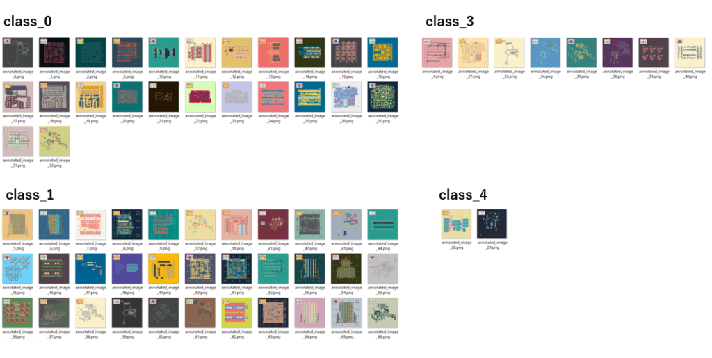
print("画像から特徴量を取得できませんでした。")像: annotated_image_0.png -> クラス: 0
画像: annotated_image_1.png -> クラス: 0
画像: annotated_image_10.png -> クラス: 0
画像: annotated_image_11.png -> クラス: 0
画像: annotated_image_12.png -> クラス: 0
画像: annotated_image_13.png -> クラス: 0
画像: annotated_image_14.png -> クラス: 0
画像: annotated_image_15.png -> クラス: 0
~~~~以下省略~~~~
この方法では、期待通りに分類されませんでした。
おそらく、5つのマークが類似していることや、マークの解像度が荒いことが相まって、特徴量の差があまり出なかったからだと思われます。
SIFT+BoVW+クラスタリングによる画像分類
前述の方法は、SIFTの特徴量をそのままクラスタリングしましたが、今回は SIFTで得られた特徴量からBoVWの辞書を作成し、その辞書の出現頻度をクラスタリングしてみます。
BoVW(Bag-of-Visual-Words、バッグ・オブ・ビジュアル・ワーズ)は、画像認識や画像分類の分野でよく用いられる、画像全体の特徴を捉えるための手法の一つです。自然言語処理における「Bag-of-Words(BoW)」という考え方を画像に応用したもので、画像を「視覚的な単語」の集合とみなして扱います。
具体的には、次の手順となります。
- 矩形領域の切り出し(背景画像の削除)
マークが描かれていると思われる、おおよその範囲を切り出します。 - 画像の拡大
解像度が少ないことで、特徴量が少なくなるのを避けるため、画像を3倍に拡大します。 - SIFT特徴抽出
各画像から特徴量(=特徴ベクトルの集合)を抽出します。 - BoVW辞書作成
全画像の特徴ベクトルをK-meansでクラスタリングし、分類されたクラスを辞書に登録します。 - BoVW特徴量生成
作成した辞書を使って、各画像から特徴ベクトルの出現頻度をストグラム化(L2正規化)します。 - K-meansクラスタリング
ヒストグラムの値を使って、K-meansでクラスタ分類(今回は5つ)します。 - 画像整理
分類結果に基づき、画像を対応するクラスのフォルダにコピーします。
import cv2
import numpy as np
import os
import shutil
from sklearn.cluster import KMeans
from sklearn.preprocessing import normalize
def extract_sift_features(image_folder, crop_coords):
"""
指定フォルダ内の画像からSIFT特徴量を抽出し、指定範囲を切り取って3倍に拡大して処理する。
Args:
image_folder (str): 画像が格納されているフォルダのパス
crop_coords (tuple): 切り取る領域 (x, y, w, h)
Returns:
np.array: 画像の特徴ベクトルリスト
list: 画像ごとの特徴量リスト
list: 画像ファイル名のリスト
"""
sift = cv2.SIFT_create()
descriptors_list = []
image_names = []
for filename in os.listdir(image_folder):
image_path = os.path.join(image_folder, filename)
image = cv2.imread(image_path, cv2.IMREAD_GRAYSCALE)
if image is not None:
# 指定範囲で切り取る
x, y, w, h = crop_coords
cropped_image = image[y:y+h, x:x+w]
# 切り取った領域を3倍に拡大
resized_image = cv2.resize(cropped_image, (w * 3, h * 3), interpolation=cv2.INTER_CUBIC)
# SIFT特徴量を抽出
keypoints, descriptors = sift.detectAndCompute(resized_image, None)
if descriptors is not None:
descriptors_list.append(descriptors)
image_names.append(filename)
return np.vstack(descriptors_list), descriptors_list, image_names
def build_vocabulary(descriptors, num_words=100):
"""
特徴量をクラスタリングし、視覚単語(BoVW辞書)を作成する。
Args:
descriptors (np.array): すべての画像のSIFT特徴量
num_words (int): 辞書のサイズ(クラスタ数)
Returns:
KMeans: 学習済みK-meansモデル
"""
kmeans = KMeans(n_clusters=num_words, random_state=0)
kmeans.fit(descriptors)
return kmeans
def extract_bovw_features(kmeans, descriptors_list, num_words):
"""
BoVWヒストグラムを作成し、画像特徴量を統一する。(L2正規化を追加)
Args:
kmeans (KMeans): 学習済み辞書
descriptors_list (list): 各画像のSIFT特徴量リスト
num_words (int): 辞書のサイズ(クラスタ数)
Returns:
np.array: BoVWヒストグラムのリスト
"""
image_vectors = []
for descriptors in descriptors_list:
words = kmeans.predict(descriptors)
hist, _ = np.histogram(words, bins=np.arange(num_words+1))
image_vectors.append(hist)
return normalize(np.array(image_vectors)) # ヒストグラム正規化(L2)
def cluster_kmeans(image_vectors, image_names, num_clusters=5):
"""
BoVWヒストグラムをK-meansクラスタリングで分類する。
Args:
image_vectors (np.array): BoVWヒストグラムのリスト
image_names (list): 画像ファイル名のリスト
num_clusters (int): 生成するクラスタの数
Returns:
list: クラスの割り当てリスト
"""
kmeans = KMeans(n_clusters=num_clusters, random_state=0)
kmeans.fit(image_vectors)
image_classes = kmeans.labels_
for idx, filename in enumerate(image_names):
print(f"画像: {filename} -> クラス: {image_classes[idx]}")
return image_classes
def organize_images(image_folder, image_names, image_classes, output_folder):
"""
クラスごとのサブフォルダを作成し、分類された画像を振り分けコピーする。
Args:
image_folder (str): 元の画像フォルダのパス
image_names (list): 画像ファイル名のリスト
image_classes (list): 各画像の分類クラス
output_folder (str): 結果を保存するフォルダ
"""
if not os.path.exists(output_folder):
os.makedirs(output_folder)
for idx, filename in enumerate(image_names):
class_folder = os.path.join(output_folder, f"class_{image_classes[idx]}")
if not os.path.exists(class_folder):
os.makedirs(class_folder)
source_path = os.path.join(image_folder, filename)
dest_path = os.path.join(class_folder, filename)
shutil.copy(source_path, dest_path)
print("画像の分類とコピーが完了しました!")
#=============================================================
# 実行部分
#=============================================================
image_folder = r"P:\annotated_images"
output_folder = r"P:\classified_images"
crop_coords = (50, 50, 150, 300) # 切り取り範囲
# SIFT特徴量を抽出(指定範囲+3倍拡大)
all_descriptors, descriptors_list, image_names = extract_sift_features(image_folder, crop_coords)
if all_descriptors is not None:
# BoVW辞書を構築(辞書サイズ100)
kmeans_vocab = build_vocabulary(all_descriptors, num_words=100)
# BoVWヒストグラムを取得(L2正規化付き)
image_vectors = extract_bovw_features(kmeans_vocab, descriptors_list, num_words=100)
# K-meansクラスタリングで分類(GMM → K-meansに変更)
image_classes = cluster_kmeans(image_vectors, image_names, num_clusters=5)
# フォルダに振り分け
organize_images(image_folder, image_names, image_classes, output_folder)
else:
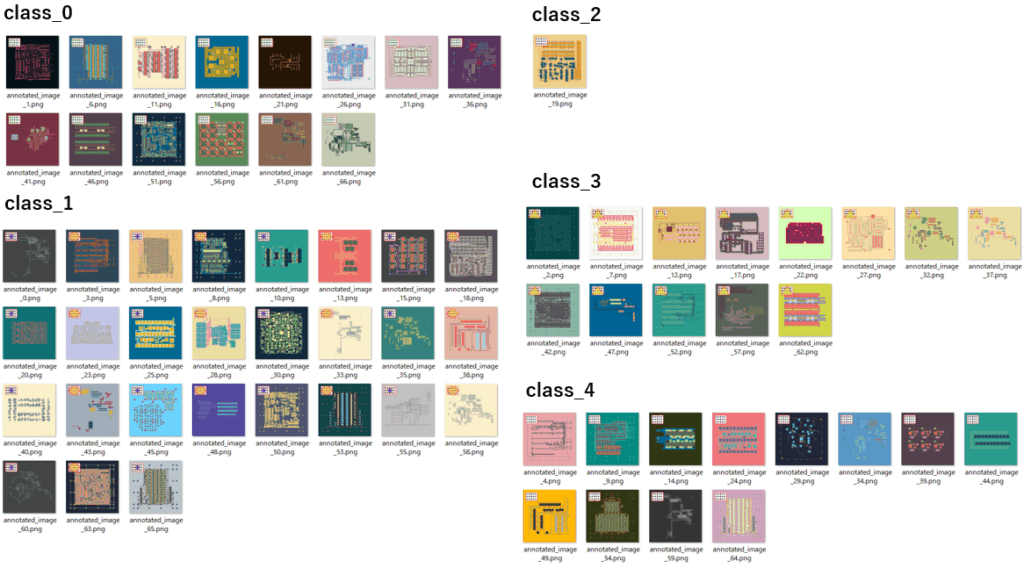
print("画像から特徴量を取得できませんでした。")画像: annotated_image_0.png -> クラス: 1
画像: annotated_image_1.png -> クラス: 0
画像: annotated_image_10.png -> クラス: 1
画像: annotated_image_11.png -> クラス: 0
画像: annotated_image_12.png -> クラス: 3
画像: annotated_image_13.png -> クラス: 1
画像: annotated_image_14.png -> クラス: 4
画像: annotated_image_15.png -> クラス: 1
~~~~以下省略~~~~
今回は、まあまあといったところでしょうか。class_0、class_3、class_4 は完全に分類できました。
class_1 と class_2 は壊滅状態なので、別途分類方法を検討したほうが良いでしょう。
まとめ
本記事では、PythonのOpenCVライブラリとSIFT(Scale-Invariant Feature Transform)を用いた特徴量ベースの画像分類手法について、基本的な処理ステップから具体的な実装方法、そして類似画像検索への応用例をご紹介しました。
SIFTは、画像のスケールや回転の変化に強く、物体認識や画像マッチングなど幅広い分野で応用されています。
画像分類の技術は日々進化しており、SIFTをはじめとする伝統的な特徴量抽出手法と、深層学習によるより高度な特徴量抽出や分類モデルを組み合わせることで、さらなる高精度な画像認識が可能になると期待されます。
本記事が、皆さんのデータ分析の一助となれば幸いです。


コメント